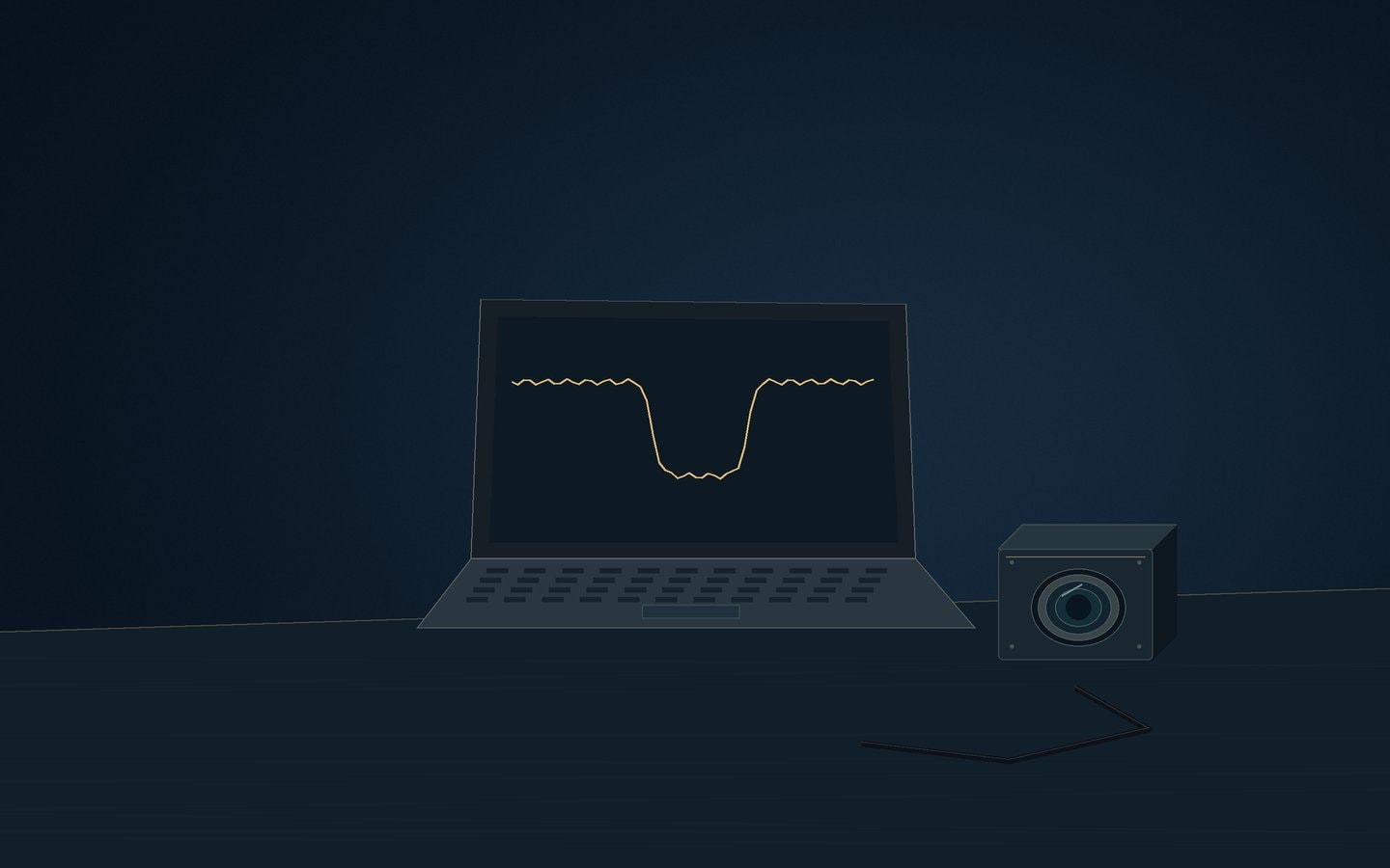
A light curve makes an occultation recording measurable. Instead of following a star only as a moving image, it shows how the measured light changes with time. Wikipedia's light-curve reference defines this as a graph of light intensity from a celestial object or region as a function of time. For an occultation, the central questions are where the light falls, where it returns, and what the recording allows those boundaries to mean.
Begin with the ordinary star signal
Look at the part of the curve before the expected event. A stable baseline gives a comparison for the dip, but real recordings have scatter. Establish the ordinary range before treating a low point as unusual. Also inspect the baseline after the event; a changed level may indicate different conditions or measurement settings.
A graph should identify the brightness quantity being plotted. Pixel sums, background-subtracted intensity and magnitude have different conventions. A magnitude scale can run in the opposite visual sense from an intensity scale, so determine which direction represents a fainter star. Check the time standard and whether plotted times refer to exposure start, middle or end. Axes that look familiar can still conceal a different measurement convention.
Wikipedia's astronomical photometry reference describes measuring the intensity of astronomical light. In image analysis, the target measurement needs a consistent area and a suitable estimate of the sky background. Nearby comparison stars help judge changes in transparency or recording conditions. They do not remove every problem automatically: blending, saturation and different positions in the field can still affect the target differently.
Read the dip in its image sequence
A straightforward asteroid event often has a transition down, a lower interval and a transition back up. The lower level can still contain light. The asteroid itself, an unresolved companion or nearby blended light can remain in the measurement area. Background subtraction also changes the numerical level. Interpret the drop relative to the surrounding star signal rather than assuming that residual light disproves an occultation.
Review the images corresponding to the transition. The target should remain in the intended measurement area; cloud, focus changes and pointing disturbances should be considered. A low point caused by the star moving outside an aperture is not the same observation as a low point while the star remains centred. Keep the original sequence available. The graph summarises the measurement, while the images explain the conditions under which it was made.
A gradual decline can have a physical interpretation, as with an atmosphere or an extended source, but it can also arise from integration. A stepped or repeated dip can suggest multiple components, yet it may be distorted by sampling or local problems. Use the shape to form a question, then test it against the recording and other stations. Do not choose the most interesting explanation solely because the curve looks unusual.
Integration changes the apparent boundary
The camera adds light over an exposure interval. If a sharp disappearance occurs within that interval, the resulting measurement mixes light from before and after the event. The plotted point may sit between the ordinary and occulted levels. This is evidence of an interval containing a transition, rather than evidence that the star necessarily dimmed slowly. Analysis should account for the exposure duration and timing convention.
Longer integration can improve the visibility of a faint target while reducing the detail of a rapid change. Shorter integration provides closer samples but may produce more scatter. The page on short asteroid events develops that trade-off. Do not make a noisy graph look cleaner by averaging away the very transition whose time is being measured. Preserve the unaveraged measurements and describe any grouping used in analysis.
Check for gaps in the sequence and repeated images. Consecutive points on a graph are not necessarily consecutive exposures. A recording or analysis step can assign an apparently even time axis to data that were not continuous. An end-to-end timestamp check with a flashing LED array addresses the relationship between recorded light and its time label. That relationship needs to be established independently of a plausible-looking event curve.
Brightness encoding also matters
Camera gain, gamma and saturation affect the relation between incoming light and saved values. A display adjustment can change how a video looks without changing the underlying measurements, while an adjustment applied inside the camera can alter the recorded signal itself. Learn which kind of operation is being used. The page on camera response testing explains why a photometric interpretation needs attention to that distinction.
The event time and its uncertainty should reflect the evidence. A sharp, well-sampled transition may allow a stronger estimate than a shallow dip buried in scatter or partly hidden by a gap. Avoid reporting extra decimal places simply because software displays them. The analysis should state the exposure timing and the reasons for uncertainty, including any ambiguity in where the change sits within the sampled sequence.
Keep analysis connected to the report
IOTA's data-analysis section publishes member-written examinations of particular occultation observations. This reflects the work beyond recognising a dip: assumptions, equipment behaviour and combined results may need detailed discussion. A useful light curve remains connected to its source images, location and timing evidence so another analyst can examine the interpretation.
When preparing the observation report, state the method, event estimates, uncertainties and relevant interruptions. Preserve the curve alongside the original recording and analysis choices. A clear negative curve is also a result when the star remained measurable during the relevant interval. The goal is a brightness record that answers a physical question with an explicit timing basis.